In the fourth article of this short series we will apply our neural network framework to recognise handwritten digits.

Purpose of this article

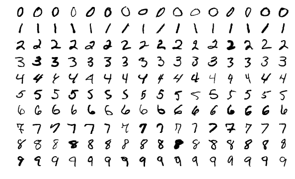
The purpose of this article is to take the neural network framework you built in the previous three articles and apply it to an actual machine learning problem. In particular, we will take the MNIST dataset – a dataset that contains images of handwritten digits – and train a neural network to be able to recognise them.

The images we will be working with are like the ones below:

By the time you are done with this article, you will have a neural network that is able to recognise the digit in an image 9 out of 10 times.

Getting the data

In the world of machine learning, the MNIST dataset is very well-known and it is common to play around with this dataset when you are experimenting with a new machine learning model. Think of it as the “Hello, World!” of machine learning.

For your convenience, I compressed the MNIST dataset it and made it available for download here (direct download link).

After you decompress the data folder, you should get two files:

• mnist_train.csv, a CSV file with 60 000 rows to train the network; and
• mnist_test.csv, a CSV file with 10 000 rows to test the network.

Each row of the file is composed of 785 integers: the first one is a number between 0 and 9, inclusive, and tells you which digit that row is. The remaining 784 integers go from 0 to 255 and represent the greyscale levels of the original image, which was 28 by 28 pixels.

Creating a new file

Because you are done with implementing the network and are now going to use it, it makes sense to create a new file for this little project, so go ahead and create a mnist.py file next to your file containing the neural network implementation.

Reading the data in

The first thing we want to do is take a look at the data, so let's go ahead and create a simple function to read it in and build a NumPy array out of the file.

In order to do that, we first use csv to import the data from the CSV file into a list with the rows of the file, and then use NumPy to convert that list of rows into an array. Do this inside the examples/mnist.py file:

import csv
import numpy as np

def load_data(filepath, delimiter=",", dtype=float):
    """Load a numerical numpy array from a file."""

    print(f"Loading {filepath}...")
    with open(filepath, "r") as f:
        data_iterator = csv.reader(f, delimiter=delimiter)
        data_list = list(data_iterator)
    data = np.asarray(data_list, dtype=dtype)
    print("Done.")
    return data

We included two extra function arguments, delimiter and dtype, to allow us to further control how csv will read the data in and how NumPy will convert the data into an actual array.

Basic data inspection

After you are done with implementing that load_data function, go to your Python REPL and take it for a spin:

>>> from mnist import load_data
>>> data = load_data("examples/mnistdata/mnist_test.csv", ",", int)
Loading examples/mnistdata/mnist_test.csv...
Done.
>>> for row in range(28):
...     if not sum(data[0, 28*row:28*(row + 1)]):
...             continue
...     for col in range(28):
...             idx = row*28 + col
...             print("#" if data[0, 1+idx] else " ", end="")
...     print()
...

      ######
      ################
      ################
           ###########
                  ####
                 ####
                 ####
                ####
                ####
               ####
               ###
              ####
             ####
            #####
            ####
           #####
           ####
          #####
          #####
          ####

In the REPL session above, we used our new function to load the test data into an array called data, and then we used a double for loop and some indexing arithmetic (idx = row*28 + col) to print the original 28 by 28 image, which is represented by 784 integers in a row inside data. We printed the very first row, if you change the 0 in data[0, 1+idx] to another integer, you will print another MNIST image.

Building the network

If we want to create a network that recognises handwritten digits, before being able to train the network we need to actually build one. For this, we will be using the components we built and implemented during the previous articles.

When building a network, two of the most important things you have to do is understand how many inputs the network should accept and how many outputs it should produce.

For our case, we have seen that the MNIST images have 784 values, so that is the number of inputs the network takes.

As for the outputs, we want the network to be able to recognise the correct digit, amongst the ten different digits that exist. For that matter, we will say that the network output will be a column vector with ten integers: the index i in the output will give a measure for how much the network thinks the input image is the digit i. If the network takes x as input and then produces the column vector out

>>> out
array([[0.40814177],
       [0.23417614],
       [0.55003812],
       [0.77545582],
       [0.83813274],
       [0.05773683],
       [0.27620492],
       [0.37310017],
       [0.47088771],
       [0.26011783]])

then we would say that, for the input x, the network recognises the digit 4, because out[4] is the largest element of out. A simple way to compute this is with np.argmax:

>>> np.argmax(out)
4

So, we have established that the network takes 784 inputs and produces 10 outputs, but how many layers does it have? And what should the learning rate of the network be? These configuration parameters are generally the things you have to tweak manually when creating a machine learning model for some task, because unfortunately there is no one-size-fits-all architecture. However, I can let you in on a little secret: for our particular case, here is a network architecture that will work just fine:

import sys, pathlib
# (Ugly) workaround to enable importing from parent folder without too much hassle.
sys.path.append(str(pathlib.Path(__file__).parent.parent))

from nn import NeuralNetwork, Layer, LeakyReLU, MSELoss

layers = [
    Layer(784, 16, LeakyReLU()),
    Layer(16, 16, LeakyReLU()),
    Layer(16, 10, LeakyReLU()),
]
net = NeuralNetwork(layers, MSELoss(), 0.001)

Of course, we cannot forget to import the relevant components from our neural network implementation, which I assumed was in a file named nn.

Testing the network

Now that we have a network, the first thing we can do is test the network to see what is the accuracy of a fresh network. If everything works out well, we expect the accuracy of this untrained network to be around 10%, which is the accuracy of a model that guesses randomly.

Testing the network is simple: go over each row of the testing data and extract the correct digit of that row and extract the 784 inputs as a column vector (this is very important, we spent the three previous articles making sure that everything would work for input vectors that were columns); feed the 784 inputs to the network; find the largest element in the output vector and compare to the correct digit; count the number of times the network guesses correctly and return the accuracy of the network:

def to_col(x):
    return x.reshape((x.size, 1))

def test(net, test_data):
    correct = 0
    for test_row in test_data:
        t = test_row[0]
        x = to_col(test_row[1:])
        out = net.forward_pass(x)
        guess = np.argmax(out)
        if t == guess:
            correct += 1

    return correct/test_data.shape[0]

This is a process that takes anywhere between a couple of seconds and a couple of minutes, depending on your computer, so let us add a print statement that shows, every one thousand iterations, how many iterations we have done:

def test(net, test_data):
    correct = 0
    for i, test_row in enumerate(test_data):
        if not i%1000:
            print(i)

        t = test_row[0]
        x = to_col(test_row[1:])
        out = net.forward_pass(x)
        guess = np.argmax(out)
        if t == guess:
            correct += 1

    return correct/test_data.shape[0]

if not i%1000 can be read as “if i has no remainder when divided by 1000”, and so it evaluates to True only when i is a multiple of 1000.

Putting everything together

If we put all the bits and pieces from this article together, and if we use pathlib to make sure we create the correct paths to the data files, this is what we have so far:

import sys, pathlib
# (Ugly) workaround to enable importing from parent folder without too much hassle.
sys.path.append(str(pathlib.Path(__file__).parent.parent))

import csv
import numpy as np
from nn import NeuralNetwork, Layer, LeakyReLU, MSELoss

TRAIN_FILE = pathlib.Path(__file__).parent / "mnistdata/mnist_train.csv"
TEST_FILE = pathlib.Path(__file__).parent / "mnistdata/mnist_test.csv"

def load_data(filepath, delimiter=",", dtype=float):
    """Load a numerical numpy array from a file."""

    print(f"Loading {filepath}...")
    with open(filepath, "r") as f:
        data_iterator = csv.reader(f, delimiter=delimiter)
        data_list = list(data_iterator)
    data = np.asarray(data_list, dtype=dtype)
    print("Done.")
    return data

def to_col(x):
    return x.reshape((x.size, 1))

def test(net, test_data):
    correct = 0
    for i, test_row in enumerate(test_data):
        if not i%1000:
            print(i)

        t = test_row[0]
        x = to_col(test_row[1:])
        out = net.forward_pass(x)
        guess = np.argmax(out)
        if t == guess:
            correct += 1

    return correct/test_data.shape[0]

layers = [
    Layer(784, 16, LeakyReLU()),
    Layer(16, 16, LeakyReLU()),
    Layer(16, 10, LeakyReLU()),
]
net = NeuralNetwork(layers, MSELoss(), 0.001)

test_data = load_data(TEST_FILE, ",", int)
print(test(net, test_data))

I ran this code once, and here is what I got:

 > python mnist.py
0.1028

The 0.1028 is 10.28%, which is in line with the accuracy we expected. Now, all there is left to do is train the network.

Training the network

Training the network is pretty similar to testing it, except that instead of comparing the network output to the correct answer and incrementing a counter for the correct answers, we need to feed the network with the vector we expected the network to output.

Building the expected output

For each row of the training data, we have information for the digit that the row actually represents, but we need to build the target column vector, the column vector we wish the neural network produced when given that same image as input. If we interpret the outputs of the network as probabilities, with the number in position i of the output representing the probability that the network gives to the input image being an i, we can reverse-engineer that to build the target output for a given image:

>>> digit = 3
>>> t = np.zeros((10, 1))
>>> t[digit] = 1
>>> t
array([[0.],
       [0.],
       [0.],
       [1.],
       [0.],
       [0.],
       [0.],
       [0.],
       [0.],
       [0.]])

Implementing training

Now that we know how to build the target column vector, we can implement our train function:

def train(net, train_data):
    # Precompute all target vectors.
    ts = {}
    for t in range(10):
        tv = np.zeros((10, 1))
        tv[t] = 1
        ts[t] = tv

    for i, train_row in enumerate(train_data):
        if not i%1000:
            print(i)

        t = ts[train_row[0]]
        x = to_col(train_row[1:])
        net.train(x, t)

Adding training to the script

Now that we have all the functions that we need, we can actually refactor our code ever so slightly to perform the network creation, testing, training and re-testing only if our script is executed directly. In order to do so, we just need the following code after all our function definitions:

if __name__ == "__main__":
    layers = [
        Layer(784, 16, LeakyReLU()),
        Layer(16, 16, LeakyReLU()),
        Layer(16, 10, LeakyReLU()),
    ]
    net = NeuralNetwork(layers, MSELoss(), 0.001)

    test_data = load_data(TEST_FILE, delimiter=",", dtype=int)
    accuracy = test(net, test_data)
    print(f"Accuracy is {100*accuracy:.2f}%")     # Expected to be around 10%

    train_data = load_data(TRAIN_FILE, delimiter=",", dtype=int)
    train(net, train_data)

    accuracy = test(net, test_data)
    print(f"Accuracy is {100*accuracy:.2f}%")

The code above prints the accuracy as a percentage (because we multiplied by 100) with two decimal places (with the :.2f inside the f-string), but other than that we just loaded the train_data in the same way we loaded the test_data array before, and we just call the train function.

I ran this code, and here is the output I obtained (after removing the intermediate prints from the test and train functions that are there just to ensure the functions are running):

 > python mnist.py
Loading mnistdata/mnist_test.csv...
Done.
Accuracy is 10.10%
Loading mnistdata/mnist_train.csv...
Done.
Accuracy is 91.94%

The exact numbers you get will probably be different, but you should get something around 10% before training the network and around 90% after training the network, provided you used the same network setup (number of layers, respective input and output sizes, respective activation functions, loss function and learning rate).

Code & next steps

You can find all the code for this series in this GitHub repository and the code that corresponds to the end of this article is available under the tag v1.1.

After reaching this point, the next sensible thing to do would be to implement a loss function that is more appropriate for this type of task, and an activation function that is more suitable to produce outputs that can be interpreted as probabilities. We will do so in the next article of the series.

If you reached this far, you may also find interesting to experiment by yourself with different network architectures and see if you can come up with a configuration that performs as well as possibly, in a consistent manner. Remember that you can change the number of layers, their internal input and output sizes, the parameter of the LeakyReLU (we have been using the default value), and the learning rate of the network.

The series

These are all the articles in this series:

1. Neural networks fundamentals with Python – intro
2. Neural networks fundamentals with Python – network & loss
3. Neural networks fundamentals with Python – backpropagation
4. Neural networks fundamentals with Python – MNIST
5. Neural networks fundamentals with Python – subtleties
6. Neural networks fundamentals with Python – student-teacher

Become a better Python 🐍 developer 🚀

+35 chapters. +400 pages. Hundreds of examples. Over 30,000 readers!

My book “Pydon'ts” teaches you how to write elegant, expressive, and Pythonic code, to help you become a better developer. >>> Download it here 🐍🚀.